RAVENFORGE

Signal & Transduction Research Log

A02 — Pickup Position and Harmonic Sampling

From normalized string coordinates to fret-dependent spatial sampling

1. Research Question — What Does Pickup Position Actually Change?

When a pickup is moved a few millimetres on the body, the first variable that changes is not “treble” or “warmth” but the spatial coordinate at which the vibrating string’s mode shape is sampled. Paiva, Pakarinen & Välimäki modeled pickup position, finite sensitivity width, and multi-pickup mixing as separable spatial effects [2], while Mohamad, Dixon & Harte showed that pickup position and plucking point can be estimated from spectral patterns in real electric-guitar recordings [3]. These results support treating pickup location as a quantifiable source of spectral signature rather than merely a subjective tone adjective.

The first audit correction in A02 is important: sin(nπx/L) for an ideal string mode is not the complete voltage response of a pickup. It is a geometric spatial factor applied to string motion. Real coil voltage additionally depends on the time derivative of string motion, magnetic-flux sensitivity, field geometry, and the downstream electrical transfer function [2,4,5]. A02 therefore addresses “where the string is read”; transduction gain and electrical filtering are passed to A03/A04.

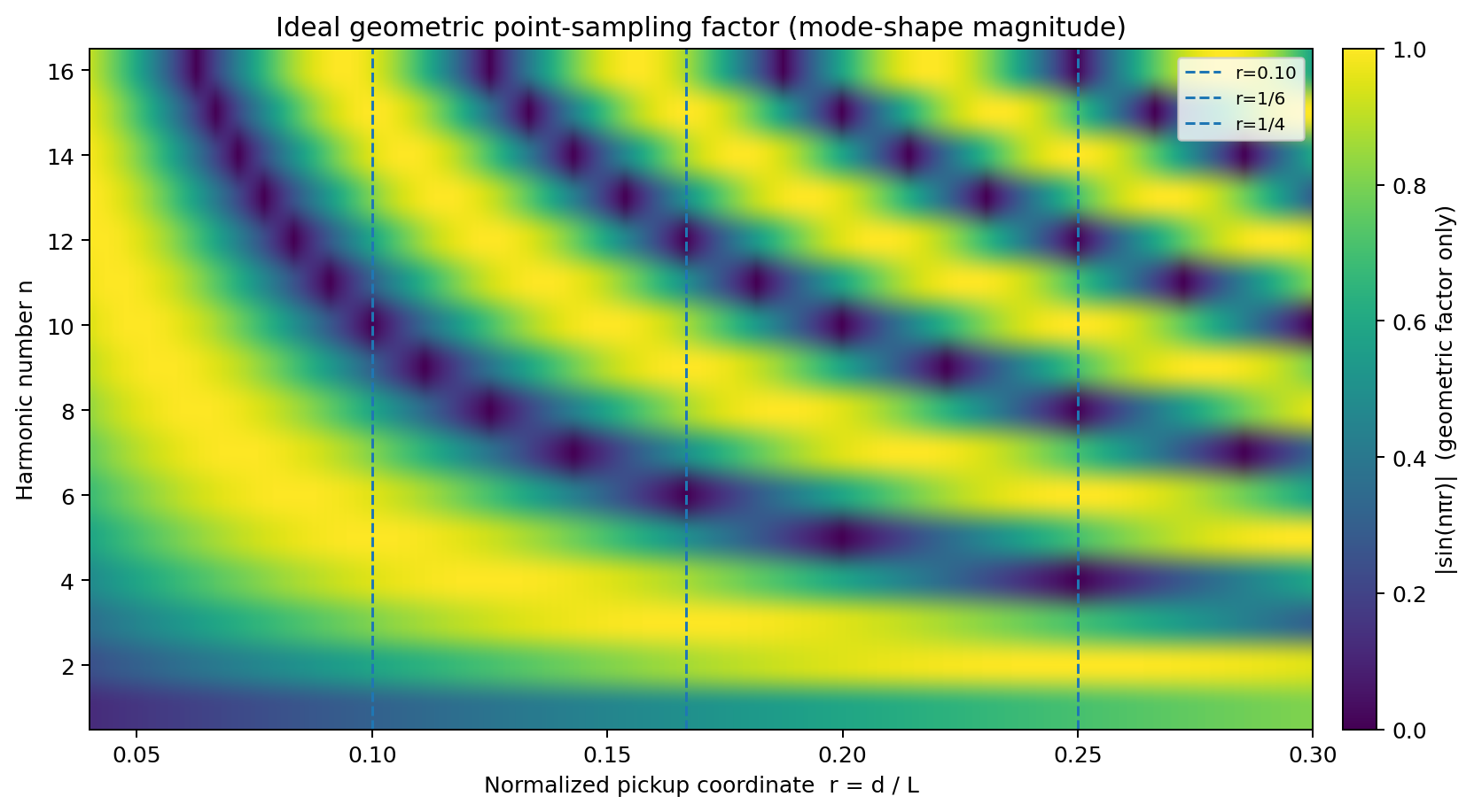
Figure 1. Geometric point-sampling factor for ideal string modes.

Color scale = |sin(nπr)|. This is a mode-shape magnitude map only — not predicted pickup voltage, EQ response, or measured RavenForge data. Dashed coordinates are examples, not recommendations [1–3].

2. Ideal Point Sampling — sin(nπr) Is a Position Factor

2.1 Coordinate Definition

To reduce coordinate ambiguity, the bridge is defined as x=0. If the current speaking length is L and the distance from the bridge to the pickup’s effective sensing center is d, the normalized pickup coordinate is r=d/L. For an ideal fixed-end flexible string, the nth transverse mode shape can be written as follows [1].

φ_n(x) = sin(nπx/L)

If an infinitesimal point sensor is assumed to read string motion at x=d, the spatial factor for mode n is [2,3]:

H_pos(n,d) ∝ φ_n(d) = sin(nπd/L) = sin(nπr)

This expression is a spatial amplitude factor. For example, if the pickup is approximated as a linearized velocity-sensitive transducer, the induced signal of the nth component additionally contains a time-derivative term approximately proportional to ω_n and a pickup-specific magnetic sensitivity. The |sin(nπr)| heatmap therefore must not be read as the actual output-voltage spectrum [2,4].

2.2 Exact Null Condition in the Ideal Model

Under the ideal point-sensor / fixed-end string assumptions, the spatial node of mode n coincides with the pickup center when n·r=m, or r=m/n, where m is an integer from 1 to n−1. For example, at r=1/4 the 4th, 8th, 12th… modes have nodes in the ideal geometric model. This relation is useful, but it does not imply that “1/4 is a good pickup position.”

3. Comb-Like Spatial Weighting — Reframing Bridge / Neck Language

Pickup-position effects are not equivalent to a conventional EQ that boosts or cuts fixed frequencies in Hz. Because the maxima and minima of sin(nπr) repeat with mode number, pickup position can be treated as comb-like spatial weighting in the harmonic domain; when combined with the modal frequencies of an actual note, that weighting appears as spectral coloration [2].

The common perception that bridge-near sampling sounds “bright” does not mean that the pickup creates high frequencies. Near the bridge, low-order transverse displacement is itself small, and the first exact nodes of low-order modes occur at more distant normalized positions; as a result, normalized upper-partial / fundamental ratios can become relatively larger. At more neckward coordinates, lower-order modes can approach a node or local minimum [2].

4. Fret Dependence — The Same Pickup Has a Different Normalized Coordinate for Each Note

Although the pickup is fixed to the body, fretting changes the speaking length. Under ideal equal temperament, the speaking length at fret F is L_F=L_0·2^(−F/12). If the bridge-referenced pickup distance d is fixed, the normalized coordinate becomes r_F=d/L_F [3].

L_F = L_0 · 2^(−F/12)        r_F = (d/L_0) · 2^(F/12)

The same pickup therefore samples a different geometric harmonic pattern on the open string, 5th fret, and 12th fret. Mohamad et al.’s fretted-note experiment likewise exploits the fact that the spectral suppression pattern of a fixed pickup changes with fret position [3]. On a real instrument, compensated saddles can make the nominal scale and actual sounding length differ slightly, so C01 uses the measured saddle-to-fret speaking length for each string.

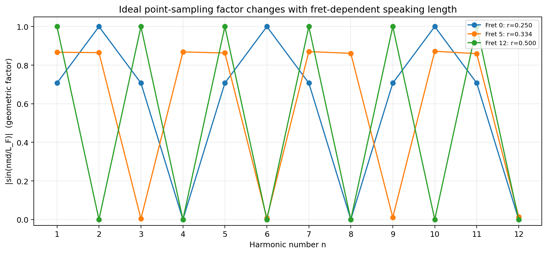
Figure 2. Different ideal geometric sampling patterns produced by the same physical pickup at different frets.

Example uses d=L₀/4 and H=|sin(nπd/L_F)|. Curves are geometric factors only, not pickup voltage. Real compensated speaking lengths must be measured per string [3].

5. Plucking Position — Separating Excitation Coordinate from Pickup Coordinate

Observed harmonic amplitude already contains the effect of excitation as well as pickup position. Following the idealized derivation of Mohamad et al., if a string is plucked at a specific point with an ideal triangular initial displacement, the nth displacement coefficient has approximately the following position dependence on the pluck coordinate ξ_q=q/L [3].

C_n ∝ sin(nπξ_q) / [n² ξ_q(1−ξ_q)]     (ideal triangular-displacement pluck)

When the point-sampling factor sin(nπξ_p) is also applied and a linearized velocity-sensitive sensor is assumed, the time derivative changes the harmonic-order envelope by one power, giving the following conceptual form. Constant terms and pickup-specific magnetic gain are omitted.

V_n ∝ sin(nπξ_q) · sin(nπξ_p) / n     (ideal string + point sensor + velocity approximation)

Plucking point and pickup point can therefore create independent spatial notches that multiply in the observed spectrum. This is why a weak harmonic in an FFT cannot be identified as a pickup node from amplitude alone. In C01, pluck coordinate, displacement, release direction, and plectrum geometry must be made repeatable.

6. Effective Sensing Width — A Real Pickup Is Not a Point Sensor

Paiva et al. model a pickup as spatially integrating string motion through a finite sensitivity function g(u) around a center P rather than sensing a single point [2]. In general form, the spatial response to mode n can be written as the following kernel integral.

H_g(n) = ∫ g(u) · sin[nπ(ξ_p + u/L)] du

For the simplest symmetric rectangular kernel, g(u)=1/W for |u|≤W/2, the RavenForge analytical baseline separates as follows.

H_rect(n) = sin(nπξ_p) · sinc[nπW/(2L)]     sinc(z)=sin(z)/z

This equation has two important implications. First, finite width averages higher-order modes more strongly, creating a spatial low-pass envelope. Second, if the kernel is linear and symmetric about the pickup center, the central ideal node defined by sin(nπξ_p)=0 remains at the same coordinate. It is therefore inaccurate to say that finite width alone shifts the node. A shifted minimum or loss of a perfect zero requires additional conditions such as field asymmetry, off-axis string position, nonlinear flux relation, 3D polarization, or non-ideal boundary/mode shape [2,4,5].

There is likewise no basis for equating physical housing width, pole diameter, or blade thickness directly with W_eff. Paiva et al. discuss center-weighted Hamming and truncated-exponential sensitivities as modeling candidates [2]. Effective sensing width is treated as a pickup-specific parameter that includes magnetic geometry, string gap, and fringe field.

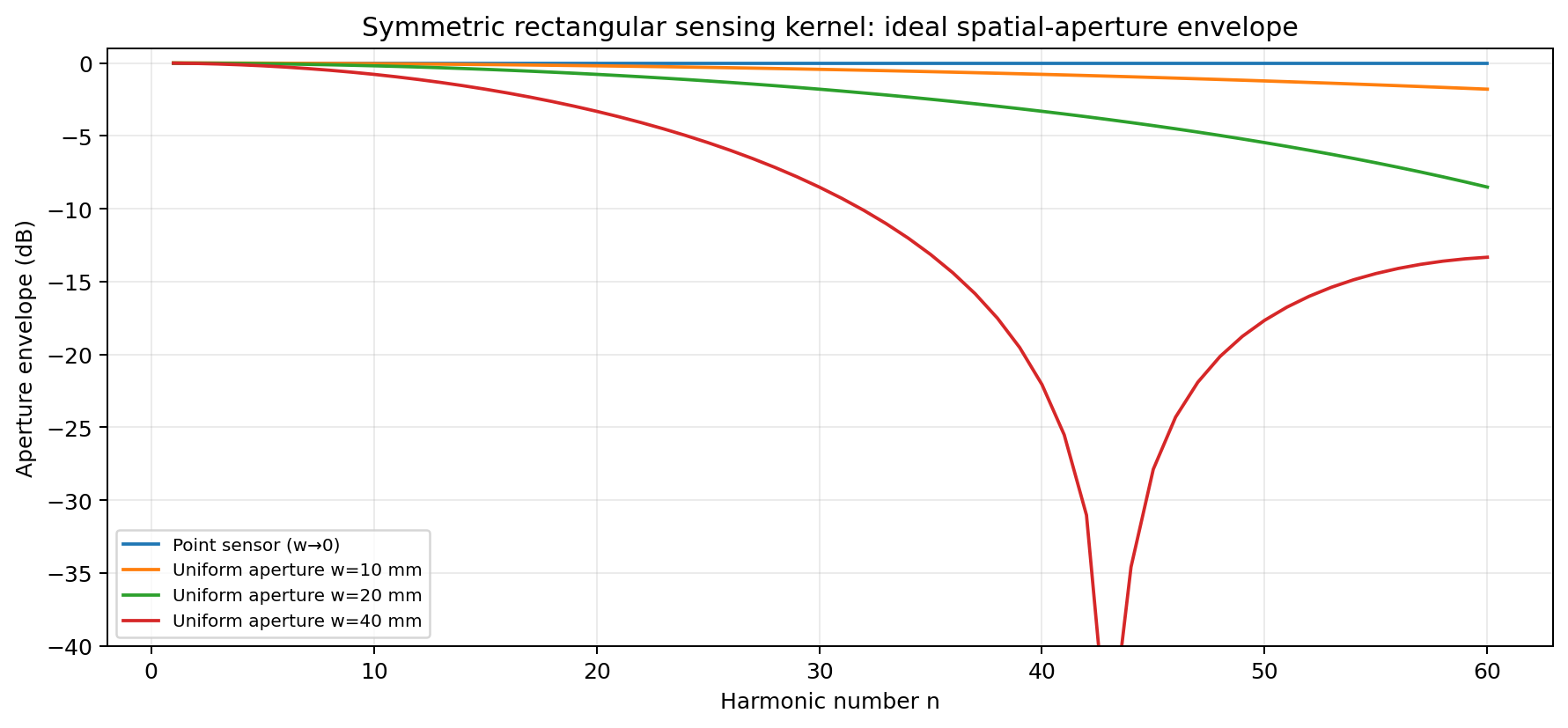
Figure 3. Idealized spatial-aperture response of a symmetric rectangular sensing kernel.

34-inch L=863.6 mm analytical example. Widths are illustrative W parameters, not measured pickup apertures. In this symmetric linear model the central position node is preserved while high-order modes are attenuated [2,3].

7. Magnetic-Field Geometry — Spatial Sampling Occurs Inside a Pickup-Specific Field

Point and finite-kernel models are useful, but the sensitivity of a real magnetic pickup arises from a 3D magnetic system formed by the permanent magnet, pole or blade, ferromagnetic string, and coil. Horton & Moore and Lemarquand & Lemarquand model how string position changes coil-linked flux through magnetic-field geometry [4,5].

String–magnet gap, pole/blade alignment, and vibration polarization are therefore confounding variables in A02/C01. Changing pickup height alters not only level but also field gradient, nonlinear response, and the magnetic force acting on the string. Feinberg & Yang experimentally and theoretically showed that a non-uniform magnetic field can split the two transverse natural-frequency modes of a guitar string [6]. Because the magnitude of this effect depends on the pickup, magnet, string, and gap, no universal numerical value is assumed.

8. Multi-Pickup Mixing — Separating Spatial Sign from Electrical Phase

If only the spatial terms of two ideal point sensors are considered, their signed mode-shape factors can combine by addition or subtraction. Assuming equal gain, equal transduction phase, and equal electrical response, the in-phase spatial baseline is:

S₊(n) = sin(nπr₁)+sin(nπr₂) = 2 sin[nπ(r₁+r₂)/2] · cos[nπ(r₁−r₂)/2]

The combined voltage of a real instrument is more complex. Pickup j contributes wiring polarity p_j, magnetic polarity, complex electrical transfer G_j(f), load, and coil phase. Conceptually, the result can be written as Y_n=Σ p_j·G_j(f_n)·H_j(n)·A_n. The phrase “out of phase = cancellation” is therefore incomplete: the degree of cancellation for each harmonic depends on both the spatial sign and the electrical phase/amplitude [2].

9. Real Strings — Do Not Confuse Inharmonicity with Spatial Nodes

Bending stiffness in a real steel string shifts modal frequencies away from exact integer multiples, producing inharmonicity [1,2]. This is an important reason why spectral notches do not sit on a perfectly harmonic Hz grid, but stiffness alone should not be described as automatically moving the spatial node coordinates of a fixed-end mode. In idealized stiff-string models, the mode shape can remain very close to sinusoidal depending on the boundary conditions; the modal frequency is the first quantity to change.

More direct routes by which real spatial mode shape and node location can deviate from the ideal prediction include non-ideal fret/nut/bridge termination, structure coupling, local stiffness, 3D or elliptical transverse motion, and asymmetric magnetic sensitivity. C01 should therefore not force every component into an exact n·f₀ FFT bin; each modal peak is tracked by a local search. The difference between the ideal node coordinate and the measured spectral minimum is stored as a separate residual.

10. RavenForge Coordinate Model — Store String × Fret × Pickup Coordinates

RavenForge does not reduce pickup geometry to a single center value on the body. For string i, fret F, and pickup j, it records the actual speaking length Lᵢ,F and the distance dᵢ,j from that string’s bridge saddle datum to its effective sensing center.

rᵢ,j,F = dᵢ,j / Lᵢ,F      Hᵢ,j,F(n) = sin(nπrᵢ,j,F)   (ideal signed spatial factor)

Under ideal equal temperament, Lᵢ,F=Lᵢ,0·2^(−F/12) can be calculated, but with a compensated bridge the measured saddle-to-fret sounding length is used. With a slanted pickup and a multiscale layout, dᵢ,j and Lᵢ,0 can both vary from string to string, so a single housing-center coordinate is insufficient to describe the layout.

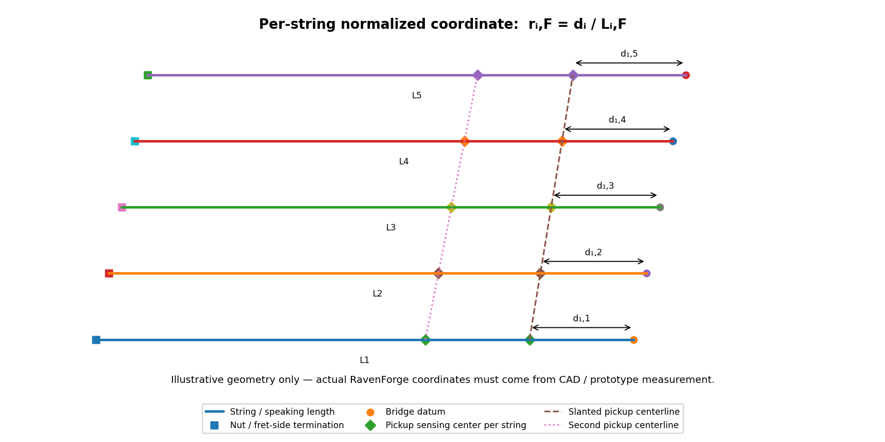
Figure 4. RavenForge coordinate definition separating dᵢ and Lᵢ for each string in a multiscale + slanted-pickup layout.

Illustrative geometry only. Slant does not automatically equalize normalized coordinates; each string requires its own measured dᵢ/Lᵢ. Actual ASKR CAD coordinates are not plotted here.

11. RavenForge Application — ASKR, EMBLA, and Future 3PU Layouts

11.1 ASKR — Treat the 37–34-Inch Multiscale as a Per-String Sampling Map

ASKR uses a different scale length for each string and a slanted pickup geometry, so the normalized coordinate can vary by string even within one housing. Instead of using a single adjective such as “bridge-near,” RavenForge builds a string × fret × harmonic map and then selects a family of CAD coordinates that best satisfies the target partial relationship defined in B02.

A02 does not invent ASKR values for dᵢ. Saddle-specific geometry is extracted from the current CAD and combined with the actual compensated speaking length to map open, 5th-fret, 12th-fret, and major low-register notes first.

11.2 EMBLA — Fret Dependence Remains Even with Parallel Frets

Even on a geometrically simpler 34-inch platform such as EMBLA, the normalized coordinate of a fixed pickup changes with fret position. RavenForge therefore does not judge “neck/bridge balance” from a single open-string fraction; it checks whether repeated deep minima occur across the registers actually used.

11.3 Future 3PU — Separate Spatial Diversity from Electrical Combination

For a 3PU system, each pickup is first evaluated with a single-pickup map to determine whether the three locations provide distinct spatial information. Pairwise and three-way combinations are then verified by combining signed spatial factors with the complex electrical transfer obtained in A03/A04. Positions are not chosen from visually even spacing or from the idea of three fixed “neck/middle/bridge characters.”

12. Evidence Matrix — Technical Audit Results Integrated

13. A02-Derived C01 Prototype Measurement Protocol

The A02 analytical model indicates what spatial effects should be expected, but a production coordinate must pass measurement repeatability. In particular, the 3.53 mm mean absolute error reported by Mohamad et al. for single-pickup position was obtained with their guitar, strings, recording setup, and inversion algorithm; it cannot be adopted as RavenForge measurement resolution or manufacturing tolerance [3]. The C01 acceptance threshold is set only after the RavenForge fixture has been characterized by R&R.

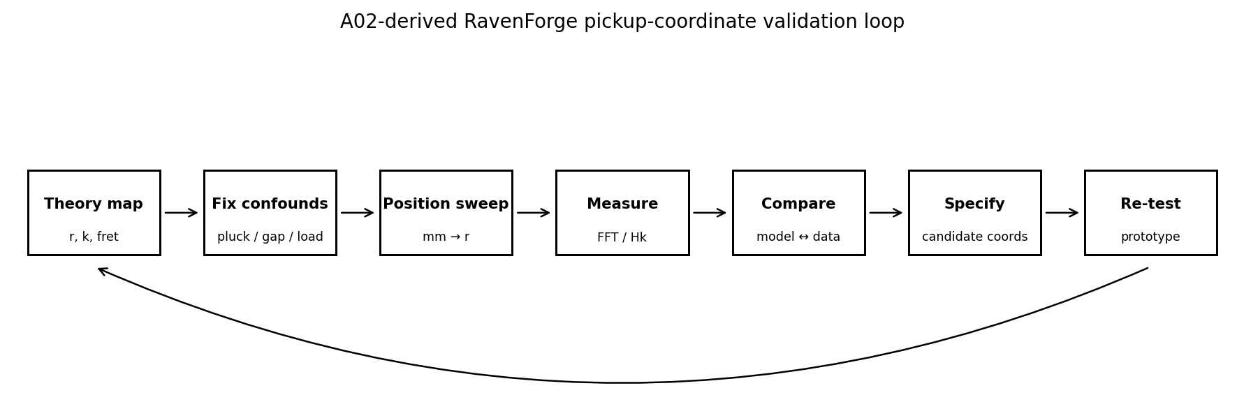
Figure 5. RavenForge pickup-coordinate validation loop derived from A02.

Engineering workflow only. The experiment must first resolve its own repeatability before millimetre differences become design specifications.

Sample rate and FFT size are measurement-design choices, not fixed requirements of the physics. RavenForge can use 96 kHz / 24-bit as a baseline, but pickup-position inference itself does not require 96 kHz. Raw waveforms are always retained, and local modal peaks are tracked using a Hann window and a sufficiently long time span. Fundamental-normalized ratios alone can become misleading when the fundamental itself lies near a spatial minimum, so absolute DI level is stored as well.

14. Current Conclusion — Pickup Position Is Conditional Spatial Sampling Geometry, Not a Single “Tone Point”

The verified A02 baseline is clear. The mode shape of an ideal string provides a spatial factor sin(nπr) at the pickup coordinate, while fretting changes the speaking length and therefore continuously changes the normalized coordinate of the same physical pickup. Plucking point is a separate excitation coordinate, and a finite sensing kernel averages higher-order spatial response. Real pickup voltage, however, results only after magnetic transduction and electrical transfer are applied to this geometric layer [2–5].

RavenForge therefore does not use “bridge / neck,” “sweet spot,” or “a few millimetres brighter” as direct design evidence. Pickup coordinates are recorded together with per-string d, actual speaking length, fret-dependent r, W_eff, gap, and combination state; a production coordinate must pass C01 repeatability and prototype measurement.

15. Next Research — What Moves to B02 and C01

References

[1] Fletcher, N. H.; Rossing, T. D. The Physics of Musical Instruments. Springer. Stretched-string modes, stiffness and musical-acoustics reference.

[2] Paiva, R. C. D.; Pakarinen, J.; Välimäki, V. “Acoustics and Modeling of Pickups.” Journal of the Audio Engineering Society 60(10), 768–782 (2012). Pickup position, sensitivity width, mixing, dispersion, nonlinear magnetic behavior and electrical response.

[3] Mohamad, Z.; Dixon, S.; Harte, C. “Pickup Position and Plucking Point Estimation on an Electric Guitar via Autocorrelation.” Journal of the Acoustical Society of America 142(6), 3530–3540 (2017). DOI: 10.1121/1.5016815. Reports 3.53 mm mean absolute error for single-pickup position under the study’s own instrument, dataset and algorithmic conditions.

[4] Horton, N. G.; Moore, T. R. “Modeling the Magnetic Pickup of an Electric Guitar.” American Journal of Physics 77(2), 144–150 (2009). DOI: 10.1119/1.2990663.

[5] Lemarquand, G.; Lemarquand, V. “Calculation Method of Permanent-Magnet Pickups for Electric Guitars.” IEEE Transactions on Magnetics 43(9), 3573–3578 (2007). DOI: 10.1109/TMAG.2007.891671.

[6] Feinberg, J.; Yang, B. “Natural-frequency splitting of a guitar string caused by a non-uniform magnetic field.” Journal of the Acoustical Society of America 144(5), EL460–EL464 (2018). DOI: 10.1121/1.5080465.

[7] Lindroos, N.; Penttinen, H.; Välimäki, V. “Parametric Electric Guitar Synthesis.” Computer Music Journal 35(3), 18–27 (2011). DOI: 10.1162/COMJ_a_00066.

[R1] RavenForge / Signal & Transduction Research Log A01. “From Mechanical Vibration to Electrical Signal.” 2026.09.05.

[R2] RavenForge internal research sequence. A02 → B02 / C01 → A03/A04 → C02.